WP3 | forward modeling and data inversion
4 octobre 2018 ( maj : 23 novembre 2020 ), par
Forward modelling
- Basic model. The most basic approximation of the ice cover on the lake is a leaky plate model of constant thickness (Stein et al, 1998), as shown in the figure below. Experience shows that, although gross at first sight, this model explains data in a surprisingly accurate fashion despite complex additional physics. It also has the advantage of having ready-to-use analytical solutions. This rapid forward model will help identifying the branches of Lamb modes propagating in the ice.
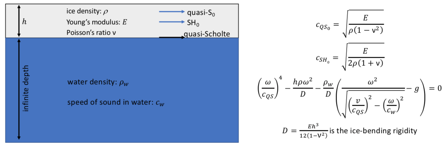
- Advanced models. Although the basic model will be useful as a first approximation, it will not be able to capture other important physics associated with the problem, such as the snow layer on the ice, the roughness of the ice to and bottom surfaces, cracks/porosity in the ice, and also the potential overall thickness variation along sensors. In view of accurate data inversion, numerical models will be developed. WP3 will be considered successful when a model, either analytical or numerical, gives a comprehensive explanation of the data. By comprehensive, we understand a model that includes the relative effects of water, ice, snow and ice damages.
Data inversion
Data inversion will consist in minimizing errors between field data and synthetic data. Agathe Serripierri, a PhD student at ISTerre is currently working on this topic. Two strategies are currently be considered.
- Inversion of the frequency-wavenumber dispersion curves of sea ice.
The noise correlation function can be calculated between every station pairsof the array. Thanks to the high spatial sampling in the main array (one meter between the 3C stations and four meters between the 1C stations), the time-space data can also be expressed in the Fourier domain, aslo known as the frequency-wavenumber dispersion curves of the ice layer. An example is shown in the following figure :
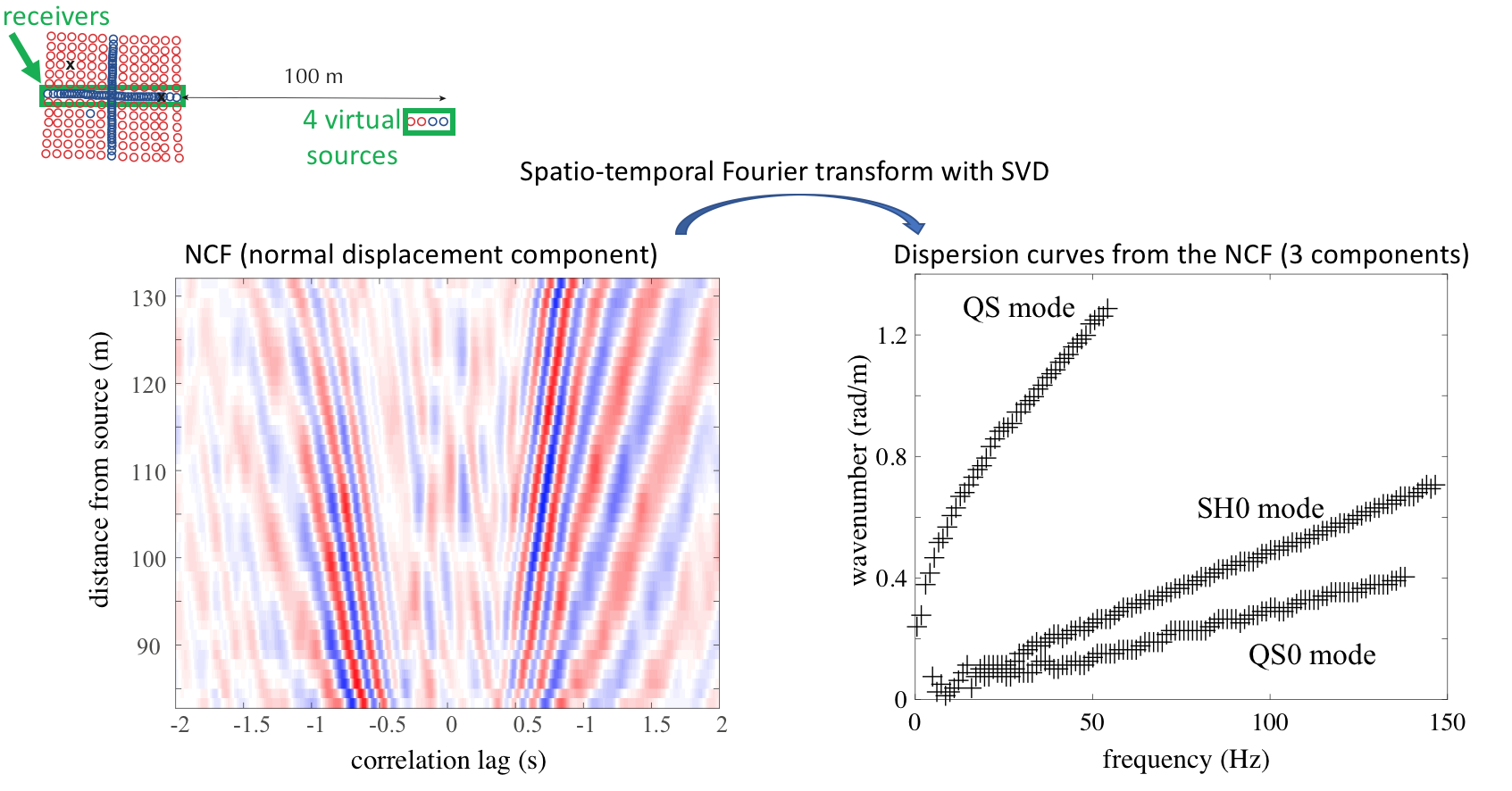
Left : NCF from the vertical channel
Right : frequency-wavenumber dispersion curves of the 3 propagating modes, obtained from the 3 displacement components
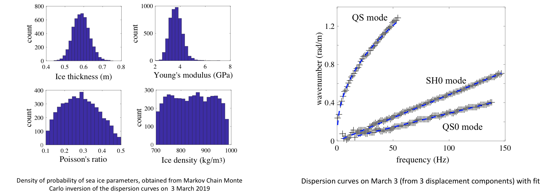
Using the forward model introduced above, it is possible to compute very efficiently the dispersion curves of the modes with any set of mechanical parameters and an ice thickness. To solve the inverse problem, we calculate the probability density function of the ice layer parameters, given the dispersion curves obtained from the data. This inversion is performed using the Markov Chain Monte Carlo (MCMC) algorithm :
This can be repeated every ay of the deployment to monitor sea ice properties :
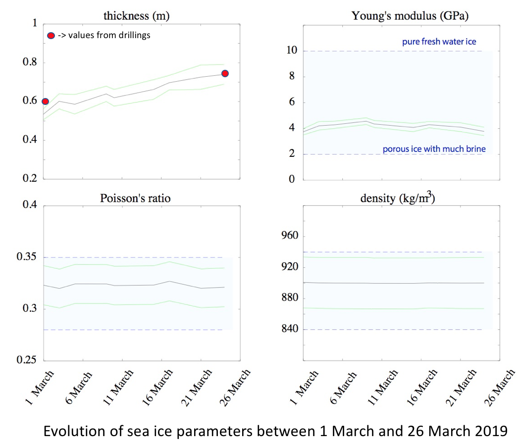
It should be noted that thickness was not constant in the fjord, so the inferred value corresponds to an average under the receivers in the dense cross of the maoin array. Nonehteless, it is consistant with values found from ice drillings, and also with values estimated from the ground penetrating radar profiles. The elastic properties are consistent with values found in literature for thin, porous first-year sea ice. The ice in the fjord was very porous in the top 30 cm, which is likely due to the presence of compacted snow at the surface.
More about this method in this paper
- Waveform inversion of icequakes.
At this point, it should reminded that the final goal of the project is the demonstration of modern seismic methods for sea ice monitoring. So far, the use of seismic methods has suffered from the difficulty of access and the challenging logistics of polar environments. It is therefore essential to reduce as much as possible the instruments required for their application. Conventional seismic methods generally require tens of geophones together with active seismic sources for monitoring applications.
The above-mentioned method, based of the analysis of the modal dispersion curves, requires about 30 stations to record the seismci wavefield, without an active source. This si already a big step forward. However, we can achieve better by considering by combining noise interferometry for estimating the elastic properties, with an inversion of the dispersion in the waveforms of the icequakes for inferring ice thickness. Thousands of icequakes are triggered every day in sea ice. They represent a very rich family of seismic signals. The following method takes advantage of the one-to-one relationship that exists between the time-frequency spectrum of the waveforms on the one hand, and ice thickness and propagation distance on the other hand.
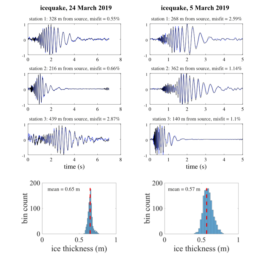
Given a Young’s modulus, E, and Poisson’s ratio, ν, the dispersion of the QS mode is characterized by a time-frequency spectrum which shape corresponds theoretically to a unique combination of ice thickness and propagation distance. A larger propagation distance results in more distorted signals with a dispersion that is specific to the ice thickness. Hence in theory it should be possible to estimate sea ice thickness based on a single signal recorded by a unique seismic station. In practice, however, this can hardly be achieved because the waveforms are corrupted by ice heterogeneity, thickness variations, the presence of a snow layer, anisotropy of elastic properties, etc. Nonetheless, the impact of these uncertainties can be mit- igated by including data from a few more seismic stations. This significantly improves source localization, which simultaneously also improves thickness estimation.
An example of waveform inversion is show in the following figure. At the tope of the figure, the waveforms of the icequakes recorded in the Van Mijen fjord are shown in black and the corresponding synthetic waveforms in blue. The inversion was performed with 3 stations only. At the bottom of the figure, the probability density function of the ice thickness is shown, with the mean value indicated as dashed line.
It is also possible to shown the probability density function fo the icequakes localization in a map :
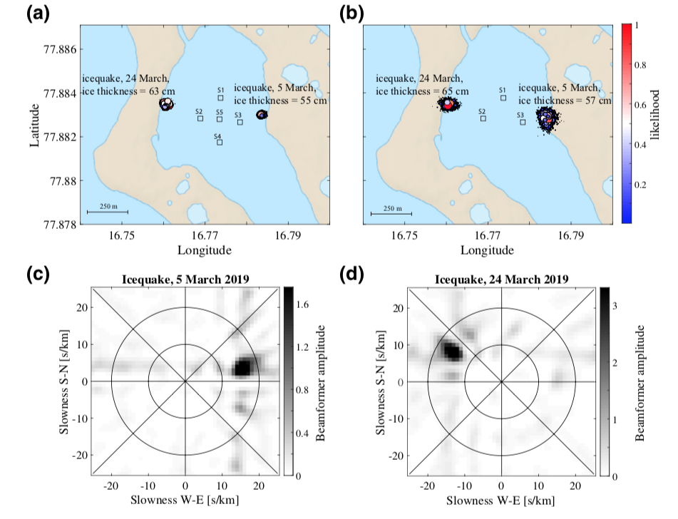
Two icequakes were inverted and shown at the top of the figure. Inversion were performed with 5 stations (a) and 3 stations (b). To check that the icequakes were properly located, we computed the slowness versus azimuth beamforming of these icequakes. The first one was recorded 5 March (c) and the second one on 24 March (d). The beamforming was computed in the 7–9 Hz frequency band, using the 231 stations of the main array.
The inferred values are consistent with those calculated from the previous inversion method. We also checked the accuracy of the localizations by inverting the active sources (jumps on the ice). The method has an impressive accuracy of less than 5 meters error, on average, on the 32 active sources positions !
This approach was also applied to another set of data recorded on drifting pack ice in 2007. Icequakes were succesfully inverted and relocated at a large ridge in the floe. Ice thickness was estimated around 2 meters, which is consistent with values found in the field from ice drillings and electromagnetic induction.
More about this method in this paper
Ice resilience observables
- Correlate damage level to ice effective properties. Once WP 1 to 3 will be completed, time-dependent variations of ice thickness and mechanical properties will be known. These variations are expected to correlate with temperature, but also with the weakening of the ice due to mechanical forcing. Consequently, the inverted mechanical properties will actually be effective properties with regard to GW propagation. As the ice reform, or heals, the effective properties will change.
- Determine parameters relevant to ice resilience. By identifying which observables are affected by damage level, it will be possible to define modelling parameters that relate to ice resilience.